From Type Design to Statistical Analysis, passing through Fourier Analysis
Part 1, Micha Wasem
Thank you very much for the introduction. My part of the talk is going to be entitled Creating Letterforms with the Fourier Transform. And of course, I should say what the Fourier Transform actually is.
Before doing so, I want to quickly remind you what a Bézier curve is, but from the perspective of a mathematician.1 Bézier curves come in different orders. The most basic case is a first order Bézier curve, which is defined from two points, P0 and P1. In this specific case, you only have a straight segment, a line, joining the two points. That’s a first order Bézier curve. And the way I like to think about this is as the trajectory of a point which is moving along the segment from one point to the other. This perspective is going to be helpful when thinking about higher order Bézier curves.
Now I’ll show you the construction of a second order Bézier curve. In this case you need more points, P0, P1 and P2, and for the construction, it makes sense to initially look at first order Bézier curves joining the points P0 and P1, and P1 and P2 respectively. As those segments are building up, you can join them by yet another moving segment like this. Finally, we’re going to let a point move on that moving segment and keep track of its trajectory. This is what gives us the second order Bézier curve. So that’s just a construction. Another way of thinking about this is that instead of moving the whole segment, you can just draw the segment four different times, let it be as it is, and then the curve that emerges traced out by all those segments is the second order Bézier curve.
I won’t talk too much about this, but I’d like to mention that if you go to third order, you have one more point, and then you do sort of an iterative construction, and it’s going to look like this.
The take-home message here, and why I’m going to speak about this, is to illustrate that if you oversimplify the situation, the basic building blocks for all of these Bézier curves is just segments of straight lines.
In order to explain in what way we go beyond Bézier, I will introduce the basic building block for Fourier.
On this slide you see a segment, and if we want to talk about the Fourier Transform, we have to replace that segment with a circle.
I should say something about the terminology here. If we speak about circles, a circle is actually defined by three pieces of information. The first is the size of the circle. You need to specify a radius. In this context, it’s called an amplitude. So we define how large our circle is. Then, because we’re looking at turning circles, we need to make sense of a notion of speed, which is going to be thought of as follows: we need to fix a time frame and count how many times the circle is going to revolve within that time frame to give us a whole number. The whole number is positive if turning counterclockwise, and negative if turning clockwise. In this example the speed will be 1, because within my time frame it’s going to turn around once. Why do we care about integer speeds and whole numbers? This is because we want the rotation to end exactly where it starts. And last but not least, we need information about an initial position, where the rotation starts in the first place.
So if we speak about a circle, we refer to a certain amplitude, speed and initial position.
The fun thing about the circles is that you can combine them. To illustrate this, I took the same circle from the previous slide, so it corresponds to the big circle here with a given initial position, with a given speed, and I attached a second circle to the first one and the second circle as you can see, is smaller, and has a different initial position. And what you don’t see, but I’m going to tell you, is that the speed is 3. So as you can see, as the big circle turns once, the small circle turns three times. The result is pretty mesmerising.
If you like, you can combine more than two circles. In this example, I took the circle with speed 1 as the biggest circle, and then, from the previous slide, we have the smaller circle with speed 3. And now I have yet a smaller circle with speed −5. So the smallest circle is going to turn clockwise five times. And you see how you have complete information on all the circles, right? You see their sizes, you see their initial positions, and I’m telling you their speeds – and yet it’s not easy to anticipate what the drawing is going to look like. To summarise, the two aspects we learn is that even though you only have three circles, the contour that results from the illustration is pretty complicated; and secondly, if you would want to draw something meaningful, you might wonder, how can I choose my circles in a specific way so that I can control the output? It’s not even a priori clear that you can draw everything you want using this method. For instance, you might think it’s not going to be possible to draw a perfect square only with circles. But we will come back to this in a minute. So one question that remains is, are there any limitations for what we can draw in this way? And the second question is, how do we choose circles wisely in order to draw something that looks good?
To try and summarise this, we can observe how circles can be put together, and how they spit out a contour. And now the remaining question is whether we could arrange this the other way around i.e. to draw a specific contour, can I find a suitable collection of circles which will draw exactly what I want? The answer to this question is pretty surprising, because it turns out that you can draw everything using circles.
This is a rather deep mathematical tool devised by Joseph Fourier, which dates back some 200 years. Fourier sort of gives you the information that you can draw everything using circles, and he hands you a recipe for how to select your circles so that they will define what you want them to define. This is called the Fourier Transform.
One way to think about this is that the Fourier Transform takes a contour as an input and then it spits out a collection of circles. The only downside there is, in theory you need an infinite amount of circles. To draw a perfect square, a finite amount of circles won’t do the trick. As we will see in a minute, that’s not so bad. We’ll start from here, from a letterform ‘N’ given kindly to us by Alice Savoie, who allowed us to mess around with it. If I compute the Fourier Transform of this ‘N’, then I obtain infinite circles. And then I can just keep a finite number and recombine them to see what it creates.
For this example I’ve used 80 circles, and you can see it kind of works. I don’t claim that this is a nice letterform, but you see it’s an ‘N’. And the interesting detail maybe is that you can get a better approximation if you use more circles.
If I decide to use 200 circles instead of 80, the result is something that looks like this. It’s not perfect yet, but if you implement enough circles, then at some point you won’t be able to tell the difference from the original form – if I use 400 circles it’s already difficult to tell the difference.
So far we haven’t mentioned the aspect of creating new typefaces, as we’ve been working from an existing letterform and recreating it in a different way.
In order to show you how one can play around with this, I need to introduce the so called Fourier spectrum. If you compute the Fourier Transform, what you get is a decomposition of your contour into circles. You can apply the Fourier Transform to your contour, and the result is a collection of circles. The way I try to visualise this here is that on the horizontal axis, you have different speeds, while on the vertical axis, you have the corresponding radii of the circle. So here, for instance, you see that if you look at speed −10, you have a circle which is a bit larger than its neighbouring circles and so on. This spectrum could be seen as a sort of fingerprint of your letter.
Or to put it another way, when you have a letter, look at the corresponding spectrum, which defines what your letter is in terms of circles. In order to make this more clear, for this example I selected speeds from −20 to 20. But you can also look at a larger version of that spectrum, say from −40 to 40. What you see here is that if you move far away from 0 in terms of speeds, you see that the circles tend to become very small. This is something which happens to be universally true. The action takes place in the middle.
To further understand what conclusions you can draw from this spectrum, I’m going to make a forward reference to Florence’s part of the talk, because she will analyse those spectra in more detail. So, what I wanted to do is to play around with that spectrum, and one option that you have is, for instance, that you say, okay, I’m going to compute the Fourier spectrum of a given letterform. I’m just going to leave all the circles as they are, except for one. And I’m going to change, say, the speed to 3. Then I will recombine and check the result.
As you see, if you change only one circle, it’s going to have an impact on the overall letterform. And since the frequency 3 is rather large, corresponding to a large circle, it’s a comparably slow speed, and changes the overall shape of the letter. But if you were to take a higher frequency, you see it adds more detailed modifications.
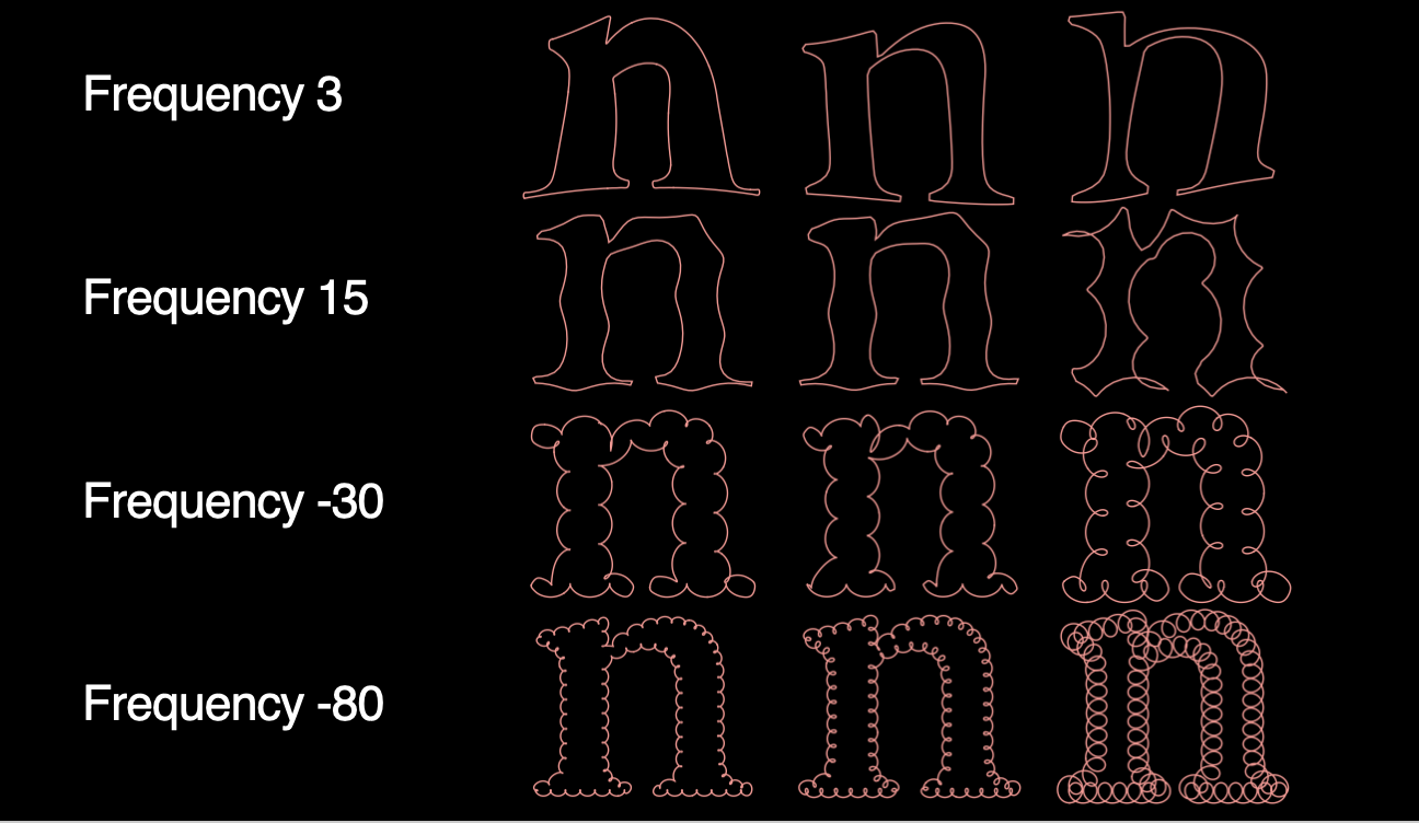
This is simply to illustrate the effects. I don’t claim again that this is useful in any way. It might give you more insight and help you to understand the effects it has. For example, if you look at a frequency −30, it results in more details at a small scale. And on the contrary, to exaggerate, a frequency −80 will give you results like on this slide.
This is only a change of one single frequency, while you could certainly think of changing multiple frequencies for even more effect. Again, I don’t say it’s useful in any way, but what it definitely is, it’s ‘Beyond Bézier’, meaning that these letterforms are not of a Bézier-type.
What I would like to speak about in the last part is a contribution of Florence and mine, because we thought Bézier already exists and we know about Fourier for 200 years… so we tried to cook up something ourselves.
We started off with the Fourier business, not with a circle but with another geometric shape. Our choice was a so-called triangle of constant width, a geometric shape which shares a property with the circle, namely that if you squeeze it in between two parallel lines, these lines will be a certain distance ‘d’ apart. Interestingly, if you do the same with two other parallel lines touching the form, but oriented in a different way, they will always also be distance ‘d’ apart. So no matter how you do it, it’s always going to be distance ‘d’.
To explain this mathematically, we’ll look at two formulas:

That’s the first one. Mathematically, replacing the circle in the whole Fourier story with triangles of constant width, comes down to replacing a term by something similar but more complicated. The main point I want to make here is that it depends on a certain parameter ‘a’. And what you might see in the formula is if that ’a’ is actually 0, then you don’t actually replace anything at all. So if ‘a’ is 0, you really have a circle. And if I increase ‘a’, the shape is going to become a triangle of constant width, which is still kind of similar to the circle.
As I increase ‘a’ further, it becomes more and more different from the circle.
The reason why I coloured this 1/8 is because that’s actually the last value for ‘a’ where you still have this kind of triangle with constant width. And if you increase the value, you end up with a weird curve with ’self-intersections’. I continue drawing these for a reason, because if you increase ’a’ more and more, it gets worse. As it turns out, to my own surprise, that if you do the whole mathematics for the Fourier business, the computations work as long as ‘a’ is smaller than 1/3. So even if your geometric shape is not really a triangle of constant width anymore, the math makes sense until you arrive at a slightly smaller number than 1/3. And we thought that it might be fun to look at a geometric building block with self-intersections.
For the next slide I decided ‘a’ to be 1/8. So that’s the borderline case where it’s still a triangle of constant width. You can combine these in much the same way that you can combine circles – and they’re going to draw shapes for you. Again, we tried to decompose a letter form using these forms instead of circles and again we abused a letterform by Alice Savoie. So here’s the S as it should be.
If you look at an approximation with triangles of constant width, you see that it’s very rough, even wild, which in a revealing way addresses the criticism that using Bézier curves in the design process produces letterforms which are too clean. This is anything but clean, that’s for sure.
Additionally in this context, you gain a certain spectrum which tells you how large your triangles of constant width need to be, and at what speeds they have to maintain, and so on. In the end the required spectrum turns out to be the Fourier spectrum of a suitable modification of your letter. So the modification R takes your letter S and turns it into something super wobbly and nasty. But it turns out that the Fourier spectrum of that weird, bizarre thing is actually the spectrum of S with respect to those triangles.
The last experiment we did is studying the transformation R, a transformation which can be reversed. It can be applied back and forth: if you have an S, you can turn it into that wobbly thing, and you can reverse the process. In this case, this specific R to the minus one, which is the inverse of R, is pretty easy to compute.
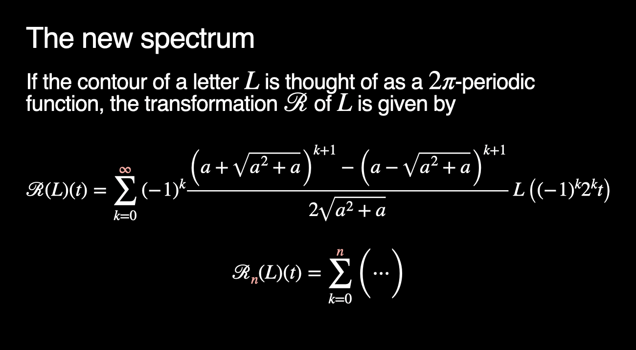
Unfortunately, as you can see from this formula, R itself has a rather untelling expression. The only reason why I include this formula in the presentation is the pink infinity sign. It would go too far to explain what that exactly means, but it is a sum involving infinitely many terms. And of course, if you apply this and then you apply its inverse again, you get back to where you started from. We then thought of replacing this R by a corresponding sum, which doesn’t have infinitely many terms, but we wanted to keep track of a finite amount of them. And then, of course, if you apply this truncated Rn and then the inverse of R, you don’t arrive back to where you started, but somewhere slightly off-track.
Our last experiment was to try this combination with a value of ’a’, which was in the range where the math still worked, but the basic building block of the geometry was self-intersecting. And this led to a shape that, if I’m honest… that should be an S. The value n is pretty low, so you won’t be able to recognise what it is. But if the value of n is increased, you see it more and more resembling an S. Only now the basic building block has self-intersections, and so does this shape. And as you keep increasing n, the results get clearer and clearer. We don’t claim that this is the future S letterform. But at least, and in this we’re entirely certain, it’s not at all of a Bézier-type.
I think that’s a good point to stop and to hand over to Florence.
Part 2, Florence Yerly
Good morning. Welcome to the second part of this axis. In the previous section, Micha explained how to transform the contour of a letterform into numerical information using the Fourier Transform. That’s when you have only one contour and then end up with numbers for an amplitude associated to each speed, to the frequency. For each letter then, you have a collection of rotating circles at different speeds. Each speed is denoted by its frequency associated with the radius of a circle. This graph shows the frequency and the radius, the amplitude.
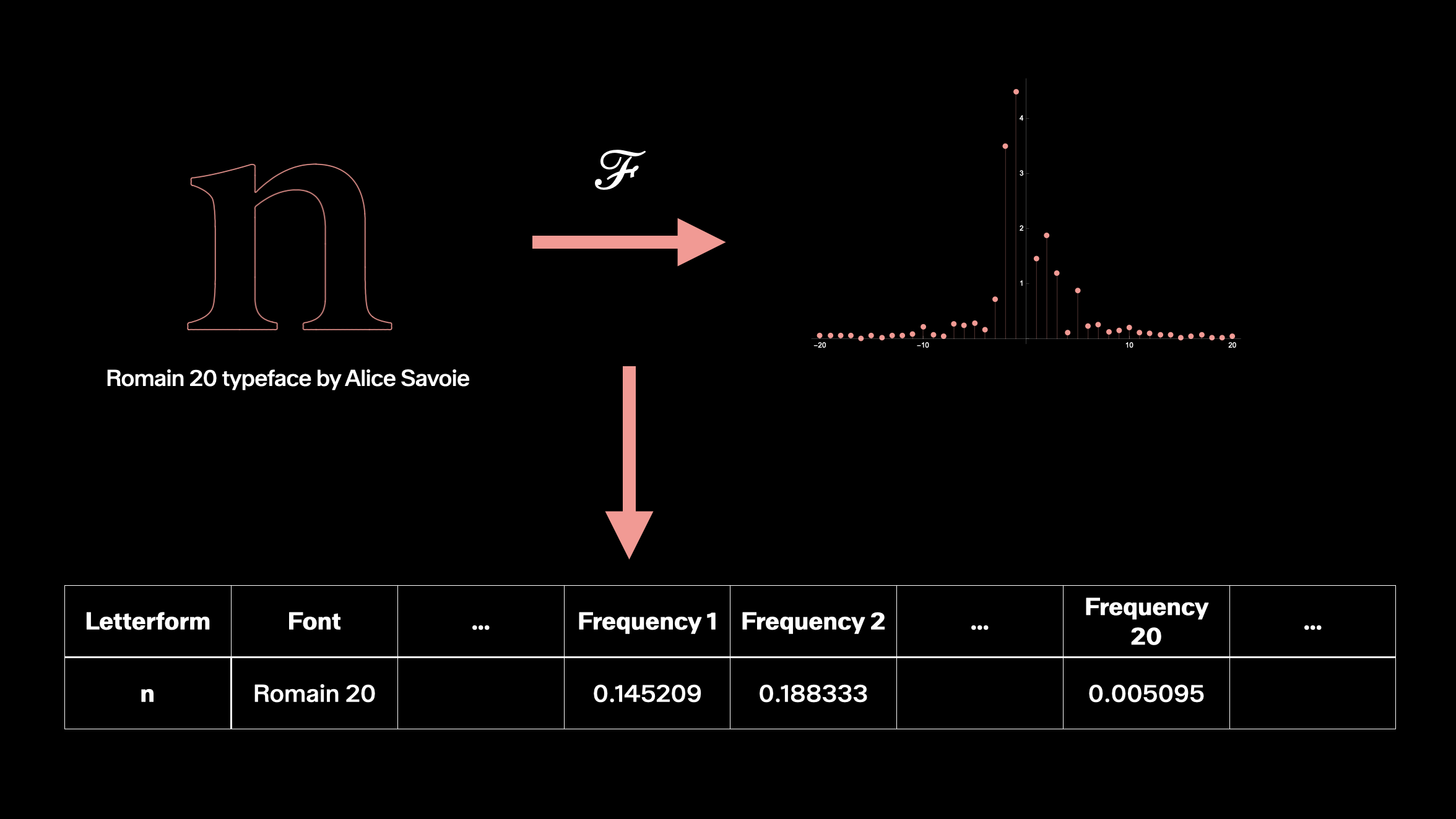
As for me, I see a line in an Excel file – because I have the information for the N from the font Romain 20, and I have these columns with each frequency and associated amplitude. Remember that for high frequencies, you have small numbers, small quantities, details for the contours, and for high frequencies, you have a lot of information. As I am a statistician, I thought we needed a database to try to understand whether the Fourier spectrum could give us quantitative information about typefaces. For example, does the Fourier spectrum allow us to discriminate between serif and sans-serif fonts?
As I am not a good programmer, I consulted with Beat Wolf, a colleague from the computer science department in Fribourg, and we came up with a Bachelor project to help us create the database. One student, Gaetan Cogliati, was interested, and he chose this project, even though it was a very different project from those which are normally on the list. And the project didn’t seem to be easy either, as it linked mathematics that wasn’t always straightforward and a field of applications that wasn’t very common. In the end Gaetan was able to create a database with 100 different fonts. And now we can automatically calculate the spectrum for all letters with only one contour.
This is one example, and it’s important for the understanding of the following slides. Gaetan had to make a few checks to ensure the consistency of the database. Fourier Transform is a global procedure, which means if you change only one circle, it changes the overall letterform. We also had to be sure that the different font file formats led to the same result of the Fourier spectrum – which we were able to confirm.
We also had to decide to take a specific number of 1,000 points on the contour to then compute a number of 40 spectra. And we also decided to select 250 frequencies, that is 250 circles, to define the contour. To achieve a pleasing enough precision, this would be sufficient. For the high frequencies, we only have small details, so even if the accuracy is not so good, it’s perhaps not a problem to understand the letters statistically.
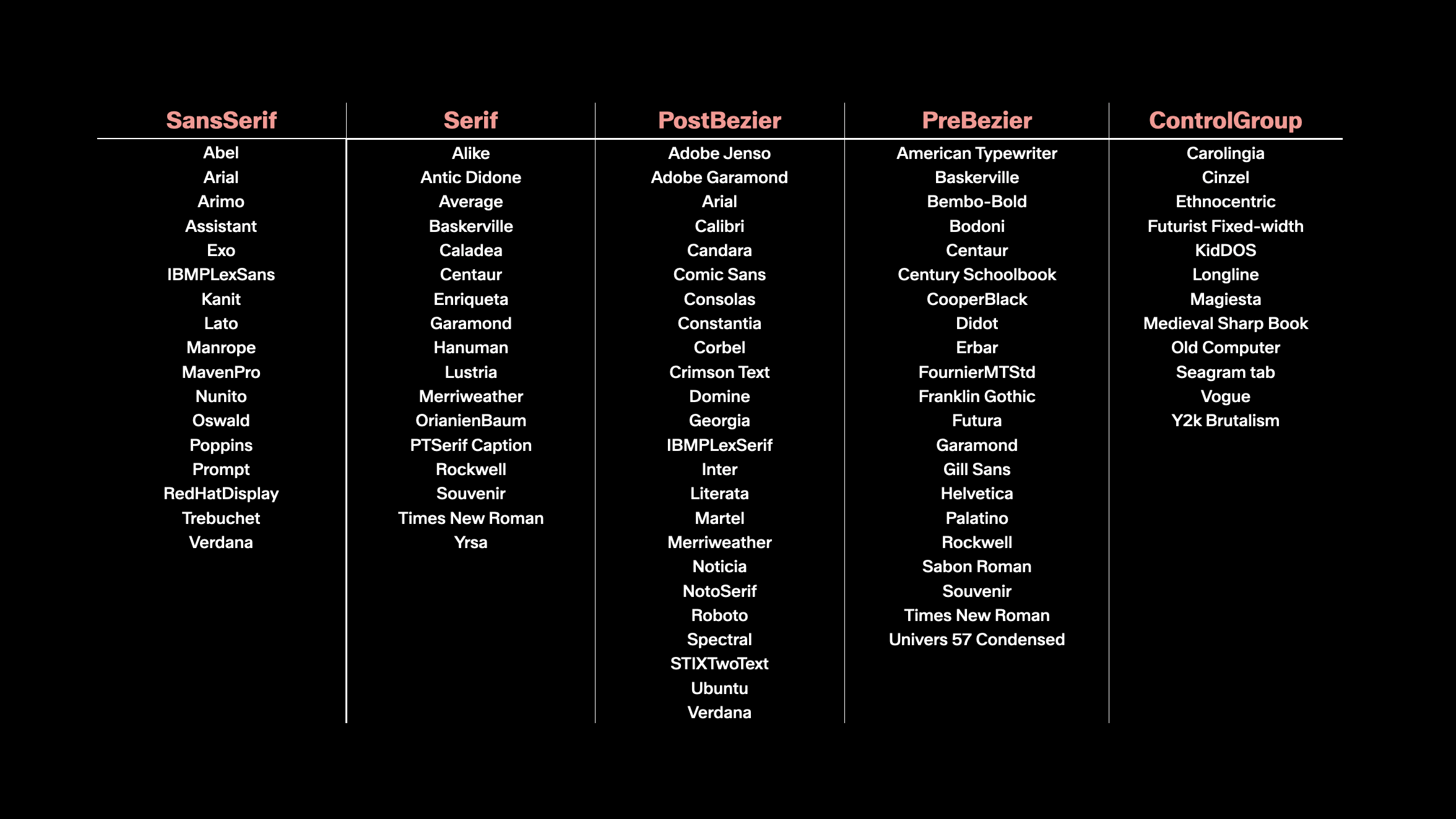
As a quick reference, here you see the fonts in the database, sorted into several groups that we thought might be of interest – sans-serif and serif are clear groups. The pre-Bézier and post-Bézier groups refer to fonts that are designed before and after the emergence of the first font editors in the 1980s, and the control group consists of fonts that are formally quite diverse.
With this database, we’re ready to dive into some statistics. Our database is an Excel file with 3,500 lines. Each line corresponds to a letterform in one font and is a point in a 250-dimensional space, which is huge. We exist in a three-dimensional space, so we can not imagine that complexity. And this is a problem. But statistics will help.
We have a tool to reduce the number of the dimensions of a set of points, called Principal Component Analysis (PCA). We can reduce the dimensions from 250 to 2, into a plane.
It’s best shown in an animation – thank you to Micha for providing this. You have this point in white there, a point in three-dimensional space, and the algorithm computes a projection of this point on the plane, so the white point in 3D will be reduced to a point in 2D.
In our case, we start in a 250-dimensional space and we reduce the information into a two-dimensional space. The algorithm takes into account that it computes the new plane, the new two dimensions, while preserving as much variability in the data as possible.
Now we are ready to see the database because we have only two dimensions. In this graph, each point, corresponds to a letter form. Here you have a lowercase w. For this graph, we limited ourselves to sans-serif fonts. And you can see immediately that some grouping emerges.
You have all the ws there, here all the ls, etc. And so the same letterforms have the same type of Fourier spectrum. If you take the capital letters, you see the brown and the blue dots are a little bit mixed, but brown and blue is w and m, similar characters, and here are G, V, U and C – U and C have perhaps the same values for the spectra as G, S, and I, so the grouping is more clear. If we change the filter of the database and choose serif fonts, the grouping is not as evident as for the san-serif fonts, but you recognise some grouping, and for the control group, we chose some forms that are quite diverse. For these, we don’t see an evident grouping, but this is not surprising.
As a first observation, we can say that PCA on Fourier spectra can discriminate the different letterforms. So, for example, an N and an S will have different Fourier spectra that allows to distinguish them just by the numbers – not regarding its contour, not its geometry, but on its numbers.
For more exotic fonts it’s more complicated, but we could make a more detailed algorithm for this.
The second question is, we can distinguish between character, but can we distinguish between serif and sans-serif fonts with the spectrum? In this first graph, we see all the characters with one contour of the serif and sans-serif fonts represented in our database, and the two groups seem very mixed. You don’t see the green dots in large parts of the graph. It’s quite spread out. But if we take all the characters, and given we just learned that each character has a specific spectra, if you then restrict the database to some letterforms, only a lowercase and uppercase S, you see that here you have the serif font, and here you have the sans-serif font. The grouping appears more clearly. The distinction between serif and sans-serif appears if we restrict the sample to only similar characters. For the M, the result is even better. And here for the I, all the serifs are there and the sans-serifs there.
In the process of the research, we presented this stage in June 2024 to our colleagues, and Radim Peško approached us to propose testing his font Mitim Sigma using our statistical analysis. So we computed the Fourier spectrum for Mitim Sigma… and you see that for the capital M, you see here pink dots for serif and green dots for sans-serif – and Mitim Sigma falls right in the middle. It’s even more clear for the L. For my non-specialist eye, this font is clearly between serif and sans-serif. I then tried with other characters of Mitim Sigma, so for F and E ,and these were clearly assigned to a sans-serif font.
In a third analysis, we wondered whether the pre-Bézier fonts covered a larger area than post-Bézier. Pre-Bézier fonts are designed before the 80s and, in our database, we have some twenty fonts. My idea was that if a set of fonts covers a smaller area than the other set, this would give us a clue that one set is more varied or less varied than the other.
The result, this graph, did not show a clear result at all. For me, all the points cover the same area. So we have no clue that pre-Bézier fonts are more or less diverse than post-Bézier. If you look at only one character here for the 7, you have one from pre-Bézier that is different from the other, but only one point is not sufficient for statistical evidence. This is a 7 from American Typewriter, just for fun. And for another character, a 2 from the same font, you see that one point differs from the others.
This was the idea of the statistics. The database is not big and we probably could go further with a larger database.
But to finish on a more creative note, not just with quantitative information, Gaetan Cogliati and the team have suggested to compute the average of Fourier’s spectrum. The idea was to choose a glyph, choose two or more fonts, and average the Fourier spectrum. So for one frequency, we have two radii and we can compute the average. With that, we can now arrive at a new Fourier spectrum for a new letterform.
We can also select the weight of each original font to create the mix. We can take fifty per cent of the first font and fifty per cent of the other – but you can also take ten or twenty per cent of Arial and eight per cent of Times. This for example is original Arial and original Times. And in the middle you have the average of the spectrum, so for example ten per cent Times and ninety per cent Arial, and in the middle it’s 50/50. It’s quite funny to see the serif appearing in the process.
Thanks to Micha, we can show an animation for the interpolation between Vogue Regular and Comic Sans. It’s also possible to make an interpretation of four fonts, as here with Oswald Regular, Times, Garamond, and Comic Sans. Right in the middle, it’s twenty-five per cent of each of the four fonts.
For the moment, I think it’s rather convincing, but, it’s really no more than a work-in-progress, because we have the Fourier spectrum only for letterforms with one contour. So far, we cannot compute the Fourier spectrum for all letters, like a B for example.
Micha and I would like to thank Gaetan Cogliati, who did a great job during his Bachelor’s degree, and I’d like to thank Beat Wolf for his expertise in machine learning. And of course, we want to thank the whole Beyond Bézier team for giving us the opportunity to work on this fascinating subject.
We also want to thank the Haute Ecole d’ingénierie et d’architecture in Fribourg for giving us the freedom to carry out the research projects that interest us. Thank you for listening.
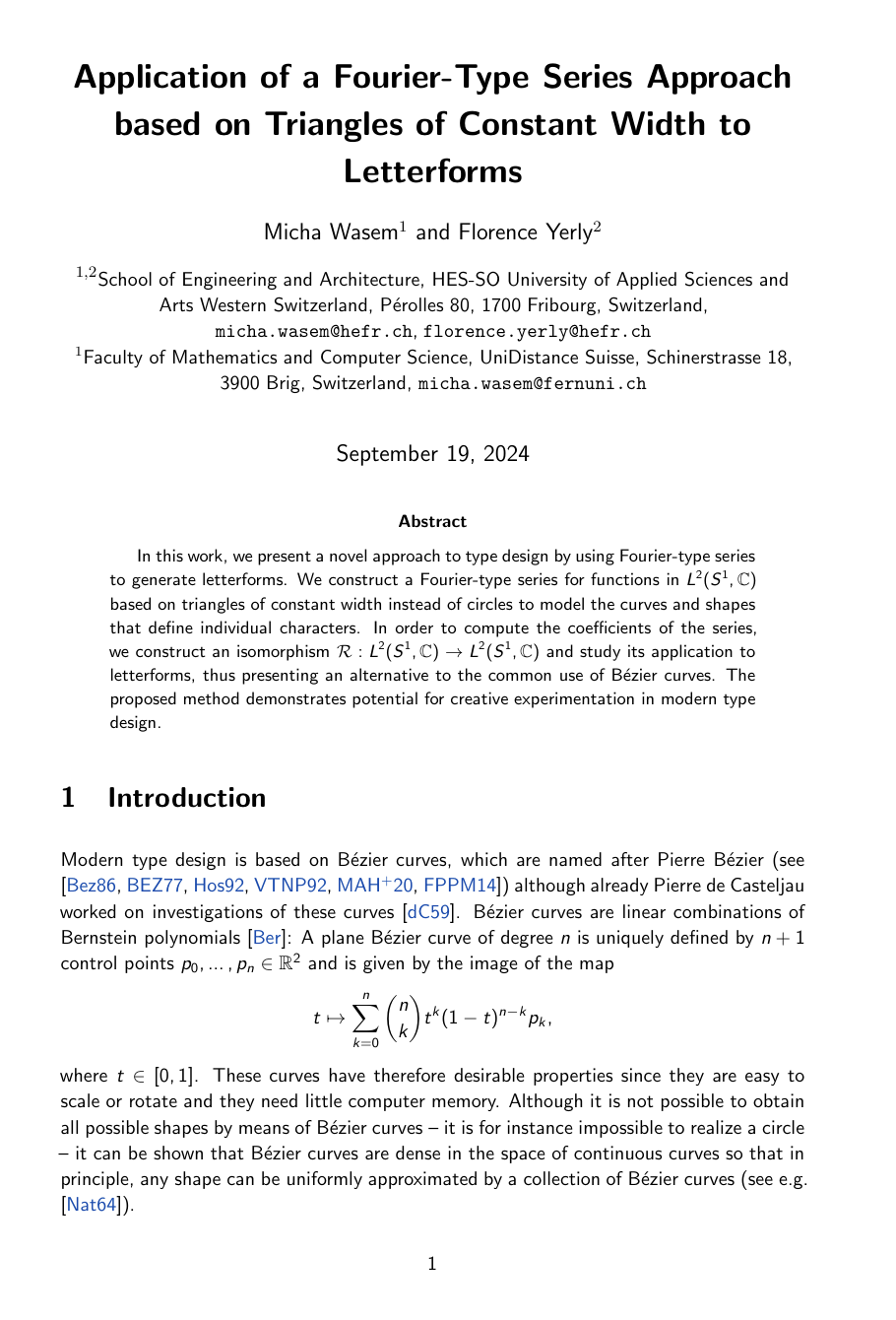
- 1 The results of this axis are also summarised in an article proposed for publication